Edgar P. Vidal, Takeshi Nagasawa
Photon Trajectories Near None-Rotating Black Holes
Abstract
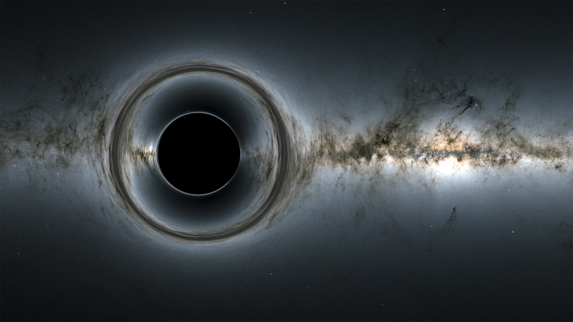
Inspired by the German physicist, Von Laue (1879–1960), who was the first person to publish a diagram showing the trajectory of light so strongly affected by gravity, we present a visualization of photons near a compact object at the 'gravitational cutoff' formally known today as a black hole. We will derive the equations of motion for a photon orbiting a black hole directly from the Schwarzchild metric. The solutions can be derived by hand to a certain point, but in our case, we opted for numerical code to solve differential equations through iterative analysis. We will not only provide diagram's of the photon orbits, but also provide an animation that displays the time dilation of a photon from an observers perspective along with source code to run it on your own computer.
Derving The Equations Of Motion and Code
Schwarzschild Metric
\[ dS^2 = -\left(1 - \frac{r_s}{r}\right)c^2dt^2 + \frac{1}{\left(1-\frac{r_s}{r}\right)}dr^2 + r^2 d\Omega^2 \]
where \(d\Omega^2 = d\theta^2 + \sin^2(\theta)d\phi^2\)
Using light \(dS^2 = 0\) and \(\theta = \frac{\pi}{2} \) such that \(d\theta = 0 \), the Schwarzschild Metric becomes:
\[0 = -\left(1 - \frac{r_s}{r}\right)c^2dt^2 + \frac{1}{\left(1-\frac{r_s}{r}\right)}dr^2 + r^2 d\phi^2 \]
"For light, the metric interval has \(dS^2 = 0\) (called a light-like, or null geodesic) and so the proper time of any light-like path is \(\tau = 0\). We thus cannot use proper-time as a parameter to describe a light-like geodesic. We can use, however, some other parameter (call it \(\sigma\)) that marks off positions along the photon trajectory. It will not be important exactly how we define \(\sigma\) here. Simply note that the constants of motion will be as before but with \(d\tau\) replaced by \(d\sigma\)". - Daniel Kasen
\(e = g_t \frac{dt}{d\sigma}\) if metric independent of \(t\)
\(\ell = g_\phi \frac{d\phi}{d\sigma}\) if metric independent of \(\phi\)
Then, we can divide our updated Schwarzschild metric by \(d\sigma^2\) to get:
\[0 = -\left(1 - \frac{r_s}{r}\right)c^2\frac{dt^2}{d\sigma^2} + \frac{1}{\left(1-\frac{r_s}{r}\right)}\frac{dr^2}{d\sigma^2} + r^2\frac{d\phi^2}{d\sigma^2} \]
Plugging in \(e^2 = \left(1 - \frac{r_s}{r}\right)^2 c^4 \frac{dt^2}{d\sigma^2}\) and \(\ell^2 = r^4 \frac{d\phi^2}{d\sigma^2}\), we get:
\[0 = -\frac{e^2}{\left(1 - \frac{r_s}{r}\right)c^2} + \frac{1}{\left(1-\frac{r_s}{r}\right)}\frac{dr^2}{d\sigma^2} + \frac{\ell^2}{r^2} \]
Multiplying through by \(\left(1 - \frac{r_s}{r}\right)\), we get that:
\[0 = -\frac{e^2}{c^2} + \frac{dr^2}{d\sigma^2} + \frac{\ell^2}{r^2}\left(1 - \frac{r_s}{r}\right) \]
\[\frac{e^2}{c^2} = \frac{dr^2}{d\sigma^2} + \frac{\ell^2}{r^2} - \frac{\ell^2 r_s}{r^3} \]
Here we have the general equation \(\frac{e^2}{c^2} = \frac{dr^2}{d\sigma^2} + V_{\text{eff}}(r)\) with:
\[V_{\text{eff}}(r) = \frac{\ell^2}{r^2} - \frac{\ell^2 r_s}{r^3}\]
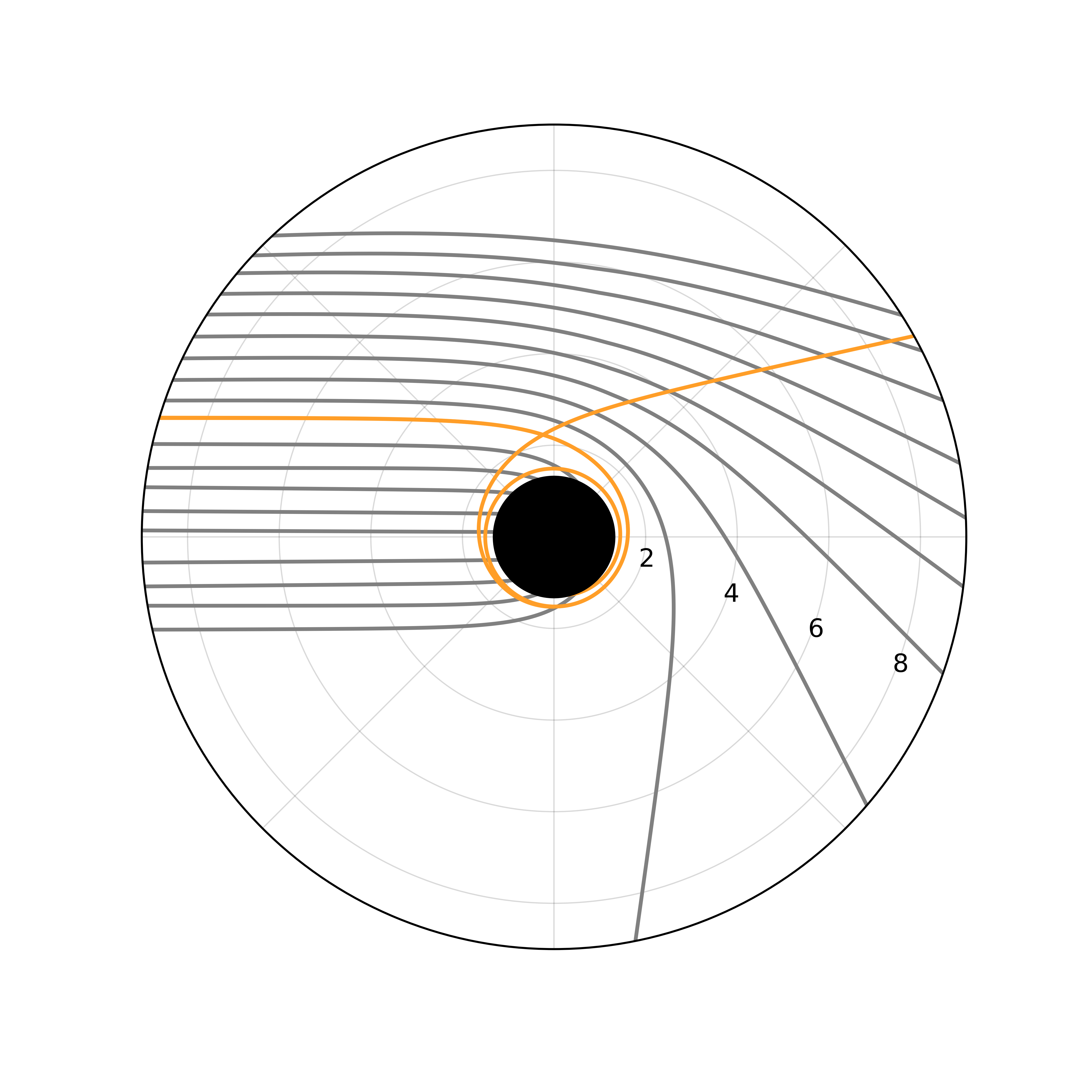
By setting \(\frac{d V_{\text{eff}}(r)}{dr} = 0\), we can find an unstable orbit at \(r_p = \frac{3}{2} r_s\). This region is known as the photon sphere and is an orbit where photons can momentarily orbit a non-rotating black hole.
Before I continue, let's define \(e\) and \(\ell\) as the specific energy and specific angular momentum. Both \(e\) and \(\ell\) are constants of motion, thus we can expect that the ratio of \(e\) and \(\ell\) are also constants of motion. Consider a photon traveling tangentially to the radius of closest approach of a black hole, such that \(\frac{dr}{d\sigma} = 0\) and \(r = r_m\) is the radius of closest approach. The metric then becomes:
\[\frac{e^2}{c^2} = \frac{\ell^2}{r_m^2} - \frac{\ell^2 r_s}{r_m^3} \]
Multiplying through by \(c^2\) and dividing through by \(\ell^2\) we get:
\[\frac{e^2}{\ell^2} = \frac{c^2}{r_m^2} - \frac{c^2 r_s}{r_m^3}\]
\[\frac{e^2}{\ell^2} = \frac{c^2}{r_m^2} \left(1 - \frac{r_s}{r_m}\right)\]
\[\frac{e}{\ell} = \frac{c}{r_m} \sqrt{1 - \frac{r_s}{r_m}}\]
We can simplify this expression by setting \(b = r_m \left(1 - \frac{r_s}{r_m}\right)^{-1/2}\) so that we write the specific energy to specific angular momentum of a photon in terms of the impact parameter \(b\).
\[\frac{e}{\ell} = \frac{c}{b} \text{ where } b = r_m \left(1 - \frac{r_s}{r_m}\right)^{-1/2}\]
Now, in order to solve the trajectory of a black hole, \(r(\phi)\), we can use the metric and use the chain rule to find a differential equation \(\frac{dr}{d\phi}\).
\[\frac{dr}{d\sigma} = \frac{dr}{d\phi} \frac{d\phi}{d\sigma}\]
\[\frac{e^2}{c^2} = \frac{dr^2}{d\phi^2} \frac{\ell^2}{r^4} + \frac{\ell^2}{r^2} - \frac{\ell^2 r_s}{r^3}\]
We already know that \(\frac{d\phi^2}{d\sigma^2} = \frac{\ell^2}{r^4}\) so we can substitute this into the metric:
\[\frac{e^2}{c^2} = \frac{dr^2}{d\phi^2} \frac{\ell^2}{r^4} + \frac{\ell^2}{r^2} - \frac{\ell^2 r_s}{r^3}\]
Now, solve for \(\frac{dr}{d\phi}\) by multiplying through by \(\frac{r^4}{\ell^2}\):
\[\frac{dr^2}{d\phi^2} = \frac{r^4}{\ell^2}\frac{e^2}{c^2} - \frac{r^4}{\ell^2}\frac{\ell^2}{r^2} - \frac{r^4}{\ell^2}\frac{\ell^2 r_s}{r^3}\]
Lastly, make the substitution \(\frac{e}{\ell} = \frac{c}{b}\):
\[\frac{dr^2}{d\phi^2} = \frac{r^4}{b^2} - r^2 - r r_s \]
Pulling out an \(r^2\) and taking the square root of both sides, we find the differential equation:
\[\frac{dr}{d\phi} = r\sqrt{\frac{r^2}{b^2} - \left(1 - \frac{r_s}{r}\right)}\]
It doesn't take too long to figure out this function is not integrable by trivial methods, so in order to find \(r(\phi)\), I will do this iteratively by setting:
\[ r = r_0 + \frac{dr}{d\phi} d\phi \]
\[ \phi = \phi_0 + d\phi \]
where \(d\phi\) is some small step \(d\phi << 1\), \(\frac{dr}{d\phi}|_{r=r_0}\), and choosing some initial conditions \(r_0\), \(\phi_0\), \(b\), \(r_s\). The challenge is to choose the right initial conditions and iterate this through the entire trajectory of a photon!
Code C161 Final Project